MFAA Chapter 9 Laboratory

LBO Valuation Engine (book §9.9)

The opening problem’s spreadsheet, rebuilt with distributions: buyout equity under EBITDA risk, multiple regimes, sweep-driven debt, and optimal exit. Organizing display: the committee panel. Seed 20260900.

import sys, numpy as np, matplotlib.pyplot as plt
sys.path.insert(0,'..')
from engine import ch09
from dataclasses import replace

1. E1 — Answer the committee

The deterministic base case sits at some percentile of the actual IRR distribution.

p = ch09.LBOParams(M=10000)
panel = ch09.committee_panel(p)
print(f"base-case IRR (deterministic): {panel['base_case_irr']:.4f}")
print(f"mean IRR: {panel['mean_irr']:.4f}, median IRR: {panel['median_irr']:.4f}")
print(f"impairment probability: {panel['impairment_prob']:.3f}")
print(f"the 'base case' sits at percentile {panel['base_percentile']:.2f} of the distribution")
print('IRR quantiles:', {k:round(v,4) for k,v in panel['irr_quantiles'].items()})

base-case IRR (deterministic): 0.1473
mean IRR: 0.0960, median IRR: 0.0926
impairment probability: 0.335
the 'base case' sits at percentile 0.61 of the distribution
IRR quantiles: {'q05': -1.0, 'q25': -0.0653, 'q50': 0.0926, 'q75': 0.2214, 'q95': 0.3896}

2. E2 — The leverage frontier

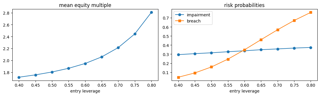
Where do the GP and LP optima diverge?

import pandas as pd
front = ch09.leverage_frontier(ch09.LBOParams(M=6000))
df = pd.DataFrame(front)
fig,ax=plt.subplots(1,2,figsize=(11,3.4))
ax[0].plot(df['leverage'], df['mean_multiple'],'o-'); ax[0].set_title('mean equity multiple'); ax[0].set_xlabel('entry leverage')
ax[1].plot(df['leverage'], df['impairment_prob'],'o-',label='impairment'); ax[1].plot(df['leverage'], df['breach_prob'],'s-',label='breach'); ax[1].legend(); ax[1].set_title('risk probabilities'); ax[1].set_xlabel('entry leverage')
plt.tight_layout(); df

	leverage	mean_multiple	impairment_prob	breach_prob	mean_irr
0	0.40	1.716328	0.294167	0.045500	0.075537
1	0.45	1.755869	0.305167	0.092667	0.076394
2	0.50	1.804289	0.314500	0.158500	0.078899
3	0.55	1.865950	0.326167	0.245000	0.084504
4	0.60	1.947023	0.336667	0.347833	0.094614
5	0.65	2.057909	0.348500	0.459333	0.112302
6	0.70	2.214107	0.357167	0.568500	0.133690
7	0.75	2.444144	0.366500	0.670500	0.161995
8	0.80	2.805829	0.373500	0.759500	0.207519

3. Closed-form validation (Proposition 9.3, lognormal limit)

b = ch09.lognormal_benchmark(ch09.LBOParams(sweep=0, mult_hot=9.75, mult_cold=9.75, regime_rate=0))
print(f"closed-form equity (BS call on EV): {b['closed_form_equity']:.2f}")
v = ch09.validation_checks()
for k,d in v.items():
    if isinstance(d,dict): print(k, 'PASS' if d['pass_'] else 'FAIL')
print('ALL:', v['all_pass'])

closed-form equity (BS call on EV): 659.88
V1_lognormal PASS
V2_deterministic PASS
V3_leverage_monotone PASS
V4_timing_value PASS
V5_reproducible PASS
ALL: True