MFAA Chapter 13 Laboratory

Exposure Switchboard (book §13.10)

The allocation cockpit: price every edge of the exposure graph, compute switching and rebalancing policies, return the policy map. Seed 20261300.

import sys, numpy as np, matplotlib.pyplot as plt
sys.path.insert(0,'..')
from engine import ch13
from dataclasses import replace

1. L2 replication (Proposition 13.3)

Smoothing-corrected beta and the Pythagoras identity.

rep = ch13.replication_report(ch13.SwitchboardParams())
print(f"beta measured {rep['beta_measured']:.3f}, corrected {rep['beta_corrected']:.3f}")
print(f"total var = spanned {rep['spanned_var']:.4f} + residual {rep['residual_var']:.4f}; TE = {rep['tracking_error']:.4f}")

beta measured 0.550, corrected 1.100
total var = spanned 0.0310 + residual 0.0100; TE = 0.1000

2. The rebalancing-band cube-root law

Band half-width scales as ε^{1/3} over decades of proportional cost.

cr = ch13.cube_root_scaling(ch13.SwitchboardParams())
plt.loglog(cr['epsilons'], cr['half_widths'], 'o-')
plt.xlabel('proportional cost ε'); plt.ylabel('band half-width'); plt.title(f"cube-root law: fitted slope {cr['fitted_slope']:.3f} (target 1/3)")
print(f"fitted slope {cr['fitted_slope']:.4f} vs target {1/3:.4f}")

fitted slope 0.3333 vs target 0.3333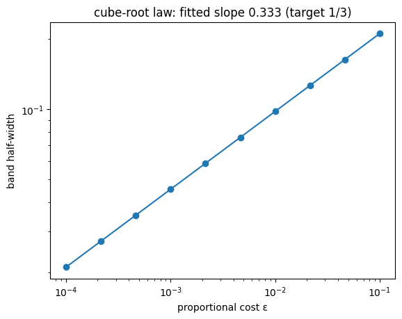

3. Optimal transport (Proposition 13.8)

Exact 1-D W₁ and Sinkhorn convergence as ε → 0.

tc = ch13.transport_convergence()
print(f"exact W1: {tc['exact_w1']:.4f}")
for r in tc['sinkhorn']: print(f"  Sinkhorn ε={r['epsilon']}: cost {r['cost']:.4f}")
print('Sinkhorn converges to the exact W1 as the regularization vanishes.')

exact W1: 0.2950
  Sinkhorn ε=1.0: cost 0.7753
  Sinkhorn ε=0.1: cost 0.3212
  Sinkhorn ε=0.01: cost 0.2953
Sinkhorn converges to the exact W1 as the regularization vanishes.

4. Validation checks

v = ch13.validation_checks()
for k,d in v.items():
    if isinstance(d,dict): print(k, 'PASS' if d['pass_'] else 'FAIL')
print('ALL:', v['all_pass'])

V1_replication PASS
V2_cube_root PASS
V3_transport PASS
V4_w1_shift PASS
V5_hysteresis PASS
V6_reproducible PASS
ALL: True